This page is automatically generated from a Jupyter Notebook.
Download the original notebook using the button below.

Download Notebook

---

Calibrating your Detector for Energy Response

Introduction

Experimental Set up

Experimental Item	Description
Detectors	2x Scionix 38 B 37 1.5M - E1 PMT
Detector Bias	500 Volts (for both)
Source Type	Spectrum Techniques Cs137
Source Activity	5 uCi
Source Manufacture Date	May 2017
Source Half Life	30.1 yrs
Cables	50 Ohm LEMO - 10ns length
Vireo Input Termination	50 Ohm

add picture of setup

add Diagram of setup

Calibrating your Detector for Energy Response (Cs137)

Setting up Environment

We’re going to define some variables up front so they are easier to change later. TRIGGER_SENSITIVITY defines how sensitive the trigger is to capture a pulse. NUMBER_OF_EVENTS indicates how many events we are going to capture before stopping data collection

---

Collecting Data

%matplotlib inline
import skutils
import math
import numpy as np
import matplotlib.pyplot as plt
import scipy

plt.rcParams["figure.figsize"] = [20, 9]

# VIREO_URL = "192.168.128.154"
VIREO_URL = "vireo-000019.tek"
# VIREO_URL = "192.168.7.2"         # USB IP address by default if using USB - This does not change
TRIGGER_SENSITIVITY = 5
NUMBER_OF_EVENTS = 10_000
EXPERIMENT_NAME = "Cs137_Energy_Calibration"

Skutils is in beta, please contact support@skutek.com with bugs, issues, and questions

1) Connect to your FemtoDAQ Vireo

We can use the FemtoDAQController class to control our digitizer remotely in this python script. The FemtoDAQ Controller contains functions to control trigger, data capture, and recording configuration. We will use it here to configure our trigger parameters.

vireo = skutils.FemtoDAQController(VIREO_URL)
print(vireo.summary())

3) Configure Data Recording Parameters

Before capturing data, we need to configure the instrument to trigger at the appropriate level

{{EXPERIMENT_NAME}}

# load default trigger settings so we know that we're starting changing settings from a known parameter set
vireo.loadDefaultConfig()

# Configuring Trigger Settings
vireo.setTriggerSensitivity(0, TRIGGER_SENSITIVITY)
vireo.setTriggerSensitivity(1, TRIGGER_SENSITIVITY)
vireo.setTriggerXPosition(128)
vireo.setInvertADCSignal(0, True)
vireo.setInvertADCSignal(1, True)
vireo.setTriggerAveragingWindow(0, 16)
vireo.setTriggerAveragingWindow(1, 16)
# Bring baseline to roughly zero - these number will vary depending on your unit.
vireo.setDigitalOffset(0, 660)
vireo.setDigitalOffset(1, 660)

vireo.setHistogramScaling(0, 1)
vireo.setHistogramScaling(1, 1)

# Enabling Triggers
vireo.setEnableTrigger(0, True)
vireo.setEnableTrigger(1, True)

# Configuring Pulse Windows
vireo.setPulseHeightAveragingWindow(8)
vireo.setTriggerActiveWindow(32)
vireo.setPulseHeightWindow(32)

Collecting Data without Coincidence Filtering

# Configure Recording on CH0, CH1
vireo.configureRecording(
    channels_to_record=[0, 1],
    number_of_samples_to_capture=512,
    file_recording_name_prefix=EXPERIMENT_NAME,
    file_recording_format="igorph",
    file_recording_data_output="pulse_summaries",
    only_record_triggered=True,
)

# Configuring Coincidence
vireo.configureCoincidence("multiplicity", 1)

Start Waveform Capture

vireo.clearTimestamp()
vireo.start(NUMBER_OF_EVENTS)
# Wait for data to be collected up to a maximum of 5 minutes
timed_out = vireo.waitUntil(nevents=NUMBER_OF_EVENTS, timeout_time=300, print_status=True)
vireo.stop()

Vireo-000019 (http://vireo-000019.tek): collected 6753 out of 10000 events (67.5% complete) events. running time: 2.0sec
Vireo-000019 (http://vireo-000019.tek): collected 6753 out of 10000 events (67.5% complete) events. running time: 2.8sec
Vireo-000019 (http://vireo-000019.tek): collected 9999 out of 10000 events (100.0% complete) events. running time: 3.8sec
Vireo-000019 (http://vireo-000019.tek): Data Collection Complete

4) Download Data Files for Later Analysis

files = vireo.downloadLastRunDataFiles()

Vireo-000019 (http://vireo-000019.tek) Controller : downloaded `Cs137_Energy_Calibration_03.56.54PM_Apr23_2025_seq000001.itx` to '/home/skutek/app-notes/skutils-app-notes/Experiments/Cs137_Energy_Calibration/Cs137_Energy_Calibration_03.56.54PM_Apr23_2025_seq000001.itx'

5) Grab Pulse Heights from all events

First we are going to grab the pulse heights calculated by our firmware DSP.

# Skutils loader to display histogram from downloaded files
pulse_heights = []
ch0_ph = []
ch1_ph = []
for filename in files:
    loader = skutils.IGORPulseHeightLoader(filename)
    # loader = skutils.GretinaLoaderme)
    for chan_data in loader.channelByChannel():
        if chan_data.channel == 0:
            ch0_ph.append(chan_data.pulse_height)
        elif chan_data.channel == 1:
            ch1_ph.append(chan_data.pulse_height)

pulse_heights = np.asarray(pulse_heights)

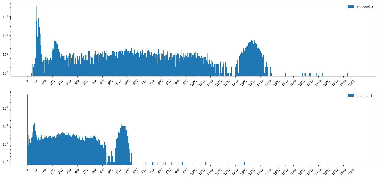
6) Calculate a histogram using Numpy

bin_width = 4
bin_edges = np.arange(0, 2000, bin_width)
hist_bins = (bin_edges[:-1] + bin_edges[1:]) / 2
hist0, edges0 = np.histogram(
    ch0_ph,
    bins=bin_edges,
)  # range=(hist_bins.min(), hist_bins.max()))
hist1, edges1 = np.histogram(
    ch1_ph,
    bins=bin_edges,
)  # range=(hist_bins.min(), hist_bins.max()))

import matplotlib.pyplot as plt

fig, axes = plt.subplots(2, 1)
axes[0].bar(hist_bins, hist0, width=bin_width, label="channel 0")
axes[1].bar(hist_bins, hist1, width=bin_width, label="channel 1")
axes[0].set_yscale("log")
axes[1].set_yscale("log")

axes[0].set_xticks(np.arange(hist_bins.min(), hist_bins.max(), step=50))
axes[1].set_xticks(np.arange(hist_bins.min(), hist_bins.max(), step=50))
axes[0].tick_params(axis="x", labelrotation=45)
axes[1].tick_params(axis="x", labelrotation=45)

print(np.sum(hist0))
print(np.sum(hist1))
axes[0].legend()
axes[1].legend()
plt.show()

9989
9819

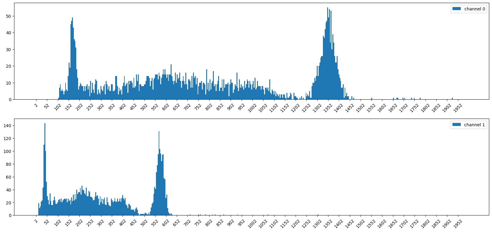
A) Define the Noise peaks by hand

\(\color{red}{\textbf{Requires User Input}}\)

noise_peak_cutoff_ch0 = 104
noise_peak_cutoff_ch1 = 12

  Cell In[1], line 5
    **Requires User Input**
    ^
SyntaxError: invalid syntax

cutoff_bin_ch0 = noise_peak_cutoff_ch0 // bin_width
cutoff_bin_ch1 = noise_peak_cutoff_ch1 // bin_width

cutoff_hist0 = hist0.copy()
cutoff_hist0[:cutoff_bin_ch0] = 0

cutoff_hist1 = hist1.copy()
cutoff_hist1[:cutoff_bin_ch1] = 0


fig, axes = plt.subplots(2, 1)
axes[0].bar(hist_bins, cutoff_hist0, width=bin_width, label="channel 0")
axes[1].bar(hist_bins, cutoff_hist1, width=bin_width, label="channel 1")
# axes[0].set_yscale('log')
# axes[1].set_yscale('log')

axes[0].set_xticks(np.arange(hist_bins.min(), hist_bins.max(), step=50))
axes[1].set_xticks(np.arange(hist_bins.min(), hist_bins.max(), step=50))
axes[0].tick_params(axis="x", labelrotation=45)
axes[1].tick_params(axis="x", labelrotation=45)

print(np.sum(hist0))
print(np.sum(hist1))
axes[0].legend()
axes[1].legend()
# plt.show()

9989
9819

<matplotlib.legend.Legend at 0x7f6a1f6540d0>

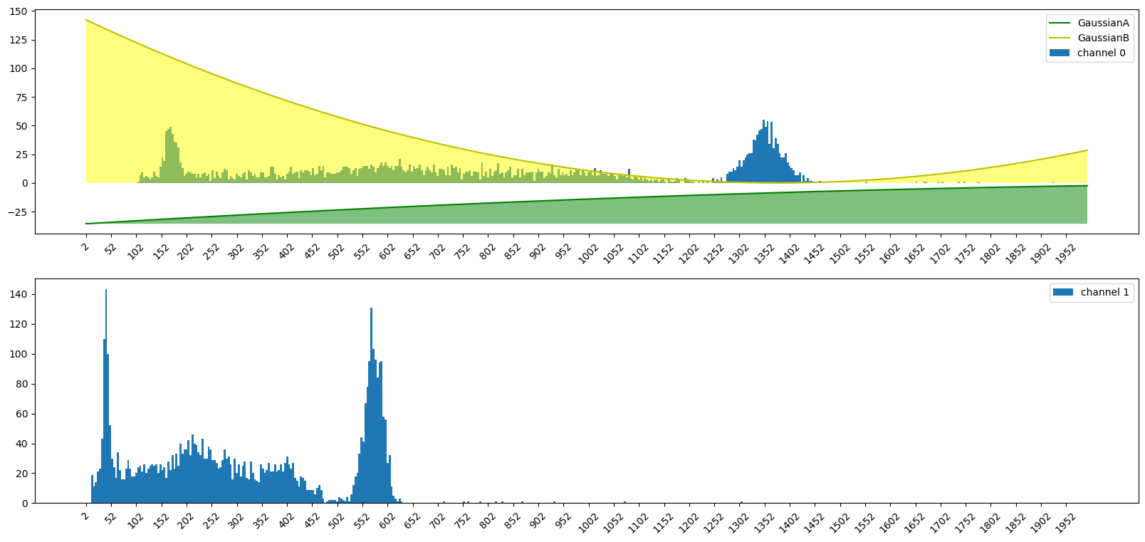
7) Finding our spectral peaks

mention the two peaks of Cs137

A) Define a two gaussian fitting function

Add More

def gaussian(hist_bins, amplitude, mean, sigma):
    result = amplitude / (sigma * 2 * np.pi) * np.exp(-0.5) * ((hist_bins - mean) / sigma) ** 2
    return result


def two_gaussians(
    hist_bins,  # raw channel histogram
    amplitudeA,
    meanA,
    sigmaA,  # fitting parameters for our first gaussian
    amplitudeB,
    meanB,
    sigmaB,  # fitting parameters for our second gaussian
):
    gaussianA = gaussian(hist_bins, amplitudeA, meanA, sigmaA)
    gaussianB = gaussian(hist_bins, amplitudeB, meanB, sigmaB)
    return gaussianA + gaussianB

A) Fit our histogram with two gaussians

Add More

ch0_2gauss_params, ch0_2gauss_covariance = scipy.optimize.curve_fit(two_gaussians, hist_bins, hist0, maxfev=100000)
ch1_2gauss_params, ch1_2gauss_covariance = scipy.optimize.curve_fit(two_gaussians, hist_bins, hist1, maxfev=100000)
ch0_2gauss_params

array([-1.36134454e-01,  2.69540747e+03,  1.38796595e+01, -3.08962083e+01,
        1.37838597e+03, -3.41140442e+01])

ch0_gaussA_amp, ch0_gaussA_mean, ch0_gaussA_sigma = ch0_2gauss_params[
    0:3
]  # grab the optimal parametets for one peak of ch0. amplitudeA, meanA, sigmaA
ch0_gaussB_amp, ch0_gaussB_mean, ch0_gaussB_sigma = ch0_2gauss_params[
    3:6
]  # grab the optimal parametets for the other peak of ch0. amplitudeB, meanB, sigmaB


ch0_gaussA = gaussian(hist_bins, ch0_gaussA_amp, ch0_gaussA_mean, ch0_gaussA_sigma)
ch0_gaussB = gaussian(hist_bins, ch0_gaussB_amp, ch0_gaussB_mean, ch0_gaussB_sigma)

# fig,(ch0_ax,ch1_ax) = plt.subplots(2)
fig, axes = plt.subplots(2, 1)
axes[0].bar(hist_bins, cutoff_hist0, width=bin_width, label="channel 0")
axes[1].bar(hist_bins, cutoff_hist1, width=bin_width, label="channel 1")
# axes[0].set_yscale('log')
# axes[1].set_yscale('log')

axes[0].set_xticks(np.arange(hist_bins.min(), hist_bins.max(), step=50))
axes[1].set_xticks(np.arange(hist_bins.min(), hist_bins.max(), step=50))
axes[0].tick_params(axis="x", labelrotation=45)
axes[1].tick_params(axis="x", labelrotation=45)

print(np.sum(hist0))
print(np.sum(hist1))

axes[0].plot(hist_bins, ch0_gaussA, "g", label="GaussianA")
axes[0].fill_between(hist_bins, ch0_gaussA.min(), ch0_gaussA, facecolor="green", alpha=0.5)
axes[0].plot(hist_bins, ch0_gaussB, "y", label="GaussianB")
axes[0].fill_between(hist_bins, ch0_gaussB.min(), ch0_gaussB, facecolor="yellow", alpha=0.5)


axes[0].legend()
axes[1].legend()

9989
9819

<matplotlib.legend.Legend at 0x7f6a1f4fd2a0>

---

Generated by nbsphinx from a Jupyter notebook.